Diffusion Maps
The 21st century is characterized by rise of massive data sets that are not only large because of sheer size but also complex due to the breadth of information they capture. Many well-established data analysis methods fail in these novel datasets due to the so-called curse of dimensionality. Diffusion maps, a method proposed by Coifman et al. [1,2,3] is a powerful tool to reduce this dimensionality by identifying the the most important dimensions in a system, which emerge as nonlinear functions of the primary data.
In contrast to linear methods such as principal component analysis (PCA), the diffusion map is a fully nonlinear method. In contrast to many other methods that are superficially similar (e.g. neighborhood embeddings) the diffusion map focusses on capturing the large-scale structure of datasets. It profits from a strong physical intuition and is fully deterministic and (in our formulation) almost parameter-free.
Diffusion maps are a broadly applicable approach, but many of their early applications were in computer science and particularly in computer vision. At BioND lab we have focused on carrying diffusion maps into applications to create social, ecological and industrial impact.
Mapping the UK Census
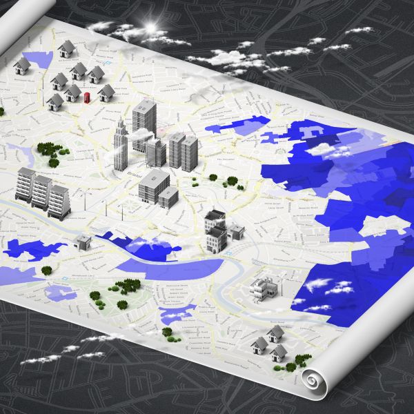
For our first trial of the diffusion map we analyzed the British 2011 Census dataset. The census is reported in terms of census output areas (COAs) which comprise 40-100 households. So in a city a COA might only be one building. For each of these COAs the census provides 1450 different statistics. However to avoid the curse of dimensionality only 50 census variable per COA are used by the office of national statistics. Instead we used the diffusion map to analyze the full census dataset for 3000 COAs around the city of Bristol [4].The diffusion map identifies new variables that describe the COAs and ranks them by importance. While the method does not provide an interpretation for these variables, some of the variables can be easily interpreted. We identified the most important variable as the "university student density". That this variable shows up as the most important emergent variable in the census (i.e. the factor that most shapes the census) is partly due to biases in the census questions. Students answer many census questions in the same way: they live with other people who they are not related to, they have A-levels but no university degree, etc.
We identified the second variable as economic deprivation. Comparing the distribution of this variable with a map of former social housing projects (council estates) yields a disturbingly accurate match. This is remarkable because the British Census does not contain income data. Instead the deprivation signal detected by the diffusion map correlates strongly with more than 600 of the census statistics, and thus picks up on the distinct living circumstances of people in economic deprivation.
Mapping the Bacterial Way of Life
Our first biological application [5] of the diffusion map was to map out the metabolic strategies employed by bacteria. We downloaded all completely sequenced bacterial genomes, identified the genes that encode known proteins and from these reconstructed the bacteria's metabolism. This gave us a good estimate of what each of the bacteria likes to eat and molecules it builds up. We then used to diffusion map to identify bacterial "lifestyle choices" i.e. the different strategies that bacteria have evolved to survive. The most important of these emergent variables distinguishes the photosynthetic cyanobacteria from all other bacteria. Apparently using photosynthesis for energy production requires a long list of dedicated adaptations of the carbon metabolism that are strongly reflected in the genome.Besides photosynthesis we find other variables that encode resource utilization strategies such sulphur reduction. Others include defenses like alcohol and acid production, cold and antibiotic resistance, and others represent adaptations to a specific habitat, such as production of biopolymers in the oceans and the production of specific molecules that are exchange with plant and animal symbionts.
Measuring Functional Biodiversity
When we talk about biodiversity we are typically interested in the diversity of ecological function that exists in a system. However, this functional diversity can be very hard to quantify. To determine the functional diversity in a system one must first know how different the species in the system are, but this is where the problems start. Typical ecological thinking starts with traits, that are morphological properties of species. These traits then determine functional capabilities which in turn determine the biogeographic distribution of a species. For many important systems we don't know the traits of the majority of species, Even if we knew them for diverse groups not all traits make sense for all species, making comparison between dissimilar species difficult.However, we show that even without knowing the traits functional diversity can be robustly quantified. Because traits ultimately determine the biogeography of a species, information on the traits is contained in the biogeographical distribution. This gives us an idea. We consider two species to be similar if they are distributed in a similar way among the samples. This naive notion of similarity has many problems, but these problems can be largely fixed by running the naive similarities through the diffusion map. The result is a method that can robustly quantify the functional diversity observed in a monitoring dataset [6].
Wifi location matching
As an industrial application of the diffusion map we solved the wifi location matching problem [7]. The latest technological revolution in Communications is the so-called internet of things (IoT). One important capability that future smart devices will need is to determine their own location. While satellite navigation can fill this need in some applications, it cannot be used indoors or in low-power devices. We particularly consider the wifi location matching problem (WLMP) where a number of devices have been installed in a number of known locations but the locations must be matched with devises based only on the wifi signal that they receive from other devices. An example of this problem is a large factory floor lit by wifi enabled light bulbs. We know where all the sockets for lightbulbs are, but we do not know which socket contains which bulb. In order to enable selective lighting of certain areas the lights must be able to determine which sockets they are installed in.To solve this problem we used the diffusion map to separately embed the sockets and the lights in a low (2 or 3) dimensional space. The matching between lights and sockets is then performed in this diffusion space, which yields 100% matching accuracy under realistic conditions and hence performs better and faster than previous methods.
The Method: Dispelling the Curse of Dimensionality
Consider again the example of the British census, where we have 1450 different statistics for every area. We can thus imagine each area as a point in a 1450 dimensional data space. This space is huge! For example it has \(2^{1450}\) corners, that's about \(10^{435}\) or in other words a good bit more than the number of atoms in the universe. Not impressed? How about the following: If you randomly placed points into this space at random and then asked what is the expected density of points exactly at a distance \(d\) from a given point, the answer that you get is that the density scales like \(d^{1449}\) -- that's a pretty steep function, if you think about it. If we randomly placed points into the 1450 almost all pairs of points would be very far apart.The curse of dimensionality appears because most pairwise comparisons that we make in a high-dimensional space compare very disparate objects, and disparate objects are hard to compare: Even in our daily lives we find it much easier to compare two songs or two paintings than comparing a song to a painting. If we make comparisons in a high-dimensional data space we are not just comparing apples and oranges, we might end up comparing an orange to world peace and the color purple.
Fortunately real data points are not randomly distributed in the high-dimensional space, they typically lie on fairly thin surfaces called manifolds. To illustrate this consider motor vehicles. There are millions of different measurements that one could take on a car, ranging from physical dimensions via the rubber composition of the tires to the absorption spectrum of the paint job. So we could think vehicles live in their own high-dimensional dataspace. But suppose I mentioned that I am thinking of a vehicle that has a gross weight of 40 tons and is 18m long. Just specifying these two dimensions gives you a good idea what kind of vehicle I am talking about. This is how manifolds work: Our data points are not all over the place, most of them are on certain narrow leaves or spines and once we know a few statistics we have a good idea which leave we are talking about and almost all the other properties of the data point can be guessed with good confidence.
The way to dispel the curse of dimensionality is to only allow comparisons between data points that are so close together that we can faithfully compare them. Since we often don't know how far comparisons are faithful we allow every point to be compared with its 10 nearest neighbors.
We can now imagine the allowed comparisons as links in a network of data points. Establishing this network enables us to make comparisons between distant points by measuring the distance on the network of allowed comparisons. The diffusion map quantifies the distances between distal points in terms of a diffusion distances, which can be conveniently computed from the eigenvectors of the Laplace matrix of the network.
The Laplacian eigenvectors also have a meaning in their own right. If we have \(N\) data points to begin with, each Laplacian eigenvector will have \(N\) elements, so each element of the vector corresponds to one of the nodes. We can say that each eigenvector assigns a new variable to each of the nodes. Since we have \(N\) such eigenvectors we get a set of \(N\) new variables for every node. In our parameterization the most important of these variables is the one which corresponds to smallest Laplacian eigenvalue that is not zero. The second one comes from the second non-zero eigenvalue and so on.
[1]
Geometric diffusions as a tool for harmonic analysis and structure definition of data: Diffusion maps
Proceedings of the National Academy of Sciences 102, 7426-7431, 2005
[2]
Diffusion maps
Applied and Computational Harmonic Analysis 21, 5-30, 2006
[3]
Diffusion maps, spectral clustering and reaction coordinates of dynamical systems
Applied and Computational Harmonic Analysis 21, 113-127, 2006
[4]
Manifold cities: social variables of urban areas in the UK
Proc. R. Soc. A. 475, 20180615, 2019
[5]
Mapping the bacterial metabolic niche space
Nature Commun. 11, 4887, 2020
[6]
Trait reconstruction and estimation of functional diversity from ecolocical monitoring data
PNAS 119, e2118156119-5, 2022
[7]
Wireless localization with diffusion maps
Sci Rep 10, 20655, 2020